Plugins, DSP, and maths for crafting acoustic soundscapes
Geometric Audio 1: Image-Source Room Models
A common audio technique for adding depth to a mix is to throw in echos or early reflections following the direct sound-source arrival to a listener. To model such reflections, many reverberation algorithms treat a sound-source and listener as a point emitter and receiver within an imaginary room or box. The reasoning follows that such a configuration is elegant from both theoretical and practical perspectives. In this series of posts, we will investigate why this is so followed by several new results that were recently derived and implemented in Riviera.
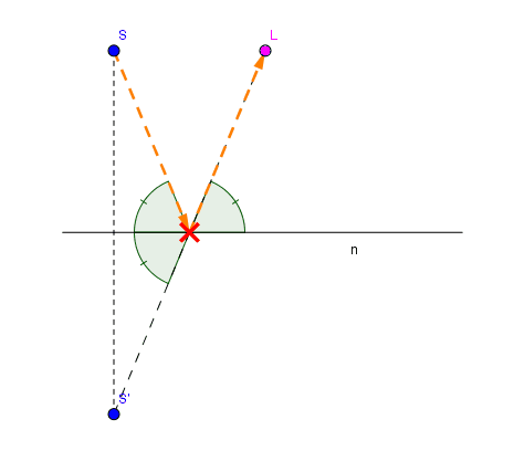
To start off, here’s an animation of a moving sound-source with respect to a listener in front of a wall. The dotted-orange line represents two rays that form the path that a sound-wave, originating from emitter , would take if it underwent a specular reflection about plane before reaching receiver .
Specular reflection model for emitter , image-source reflected across plane , and receiver
The reflection point is specific to the coordinates of and as the two incident angles of the two rays with respect to the plane must be identical. Determining follows from applying some basic high-school geometry tools. If is the “image-source” or reflection of across , then the ray will intersect at the desired point ; proof follows basic axioms of congruent angles of intersecting lines. More useful are the implications of such a construction. From the coordinates of , observe that
has length equal to the ray-traced path
Last leg of the ray-traced path is coincident to
In other words, contains useful information for computing both distance and direction of a first-order reflection (the two properties can later be used to update various DSP parameters such as time-delay, attenuation/gain coefficients, and head-related transfer functions). If the reflecting surface were to extend to infinity, then we need not even compute given that the intersection will always fall upon the surface.
A third property of the image-source construction is its extension to higher-order image-sources that preserve properties 1 and 2. Supposing that we have two planes and is the first-order image-source of reflected about . Reflecting about generates a second-order image-source shown in the animation below.
Reflecting a first-order image-source about a valid plane produces a second-order image-source
Note some of the caveats as to which planes are valid. If emitter and receiver are located within a convex enclosure of planes whose normals point inward, then the image-source must lie within the positive side of candidate plane or else the resulting ray-traced path will be physically impossible (it will pass through planes). If the candidate plane were valid and constructed, then the reflection path can be computed by iteratively back-tracing intersection points with lower-order image-sources; the total back-traced path can be shown to be equal to that of via symmetry arguments . In the example above, is the second-order intersection point between followed by the construction of ray used to find the first-order intersection point with respect to . However, if any intersection point in the back-trace were to lie outside the reflecting plane, then the entire path would be invalid (akin to a reflection off of a non-surface). This is crucial as such a check would possibly invalidate a large majority of the high-order image-sources, resulting in wasted CPU cycles. Thus we now have some hints as to the complexity of the problem space.
Supposing on average that each image-source has valid planes to reflect from (e.g. regular polygonal enclosure), then the total number of image-sources is exponential with respect to image-source order .
Only a fraction of the exponentially large set of image-sources are valid.
It should be clear now that image-source methods are computationally expensive for even well-structured enclosures so we ought to turn our attention/look towards special cases where the problem space collapses.
First, consider the case of second-order image-sources computed amongst two orthogonal planes shown in the animation below.
Second-order image-source coincident for both and . Only one back-trace path is valid at a time.
The first-order image-sources are constructed by reflecting off planes respectively. Their second-order image-sources are computed from reflecting off respectively and seem to possess coordinates coincident with respect to each (both are subsequently referred to as ). This follows from the observation that the reflections w.r.t. orthogonal and commute. i.e. reflections between orthogonal planes can be performed in any order, only their multiplicity will matter. Moreover, if we perform the back-trace from , we observe that there’s exactly one path that is ever valid with respect to a moving emitter or receiver. i.e. computing the coordinate of is sufficient as it will always have a unique non-degenerate or non-coincident valid path. How can we apply this fact to the case of rectangular room enclosures?
Let us now define a rectangular room in terms of a pair of parallel planes along dimension orthogonal to a pair of parallel planes along dimension (see the animation below). For reflections along the the dimension, only the choice of the first reflection (either or ) matters as all subsequent reflections must alternate; a one-to-one mapping exists between sequence and image-source coordinate. For reflections between orthogonal planes, the commuting property allows us to shuffle the ordering of reflections into sub-sequences restricted to those along dimension followed by those in dimension . This allows us to map any unique image-source coordinate to and from the sequence of reflections given by . Moreover, each image-source will be restricted to its image-room computed in the same way by applying the same Matrix transform to its vertex points. The result is a lattice map of image-sources within image-rooms conveniently organized along two integer axes shown below.
Integer lattice map of image-source/rooms
It should be apparent that the number of valid image-sources is no longer exponential with respect to max order reflections , but in the D case quadratic and in the general case, for dimensions. The question now arises as to whether we can do better, especially for higher dimension () where quantities grow more quickly and become non-trivial to compute.
Next posts: We determine the bounds for the number of image-sources within different radii defined under the taxi-cab distance and then the more practically useful Euclidean distance.
The taxi-cab distance on the lattice map is equivalent to the max order of image-sources. Counting the number of image-sources will bound the computations required to process individual image-sources within DSP pipelines (e.g. updating a tapped delay-line). See post. Related: linear algebra and dynamic programming
The Euclidean distance on the lattice map gives the time-interval or sampling period of which image-sources appear. Counting the number of image-sources between two distances gives an energy density or amplitude profile of an impulse response allowing us to forgo processing individual image-sources. See part 1 and part 2. Related: Gauss Circle problem, dynamic programming, and Fourier analysis
[…] for short). Normally, direct computation in these spaces is expensive but some clever maths (see tutorial) reduced the asymptotic costs to the point of practical use (e.g. a Reverb plugin). Parameterizing […]
[…] Yuancheng Luo just (02/2017) published this crazy plugin, that combines convolution and algorithmic reverb – if i get it right up to hypothetical 5 dimensions… I won’t even try to explain this black-voodoo-math-magic. Luckily there is a tutorial how to use the plugin. And if you are interested (and have some time and are capable of understanding this) he also has some background information. […]
[…] direct computation in these spaces is expensive but some clever maths [see tutorial (parts 1, 2, 3, 4)] reduced the asymptotic costs to the point of practical use (e.g. a Reverb plugin). […]


 reflected across plane


valid planes to reflect from (e.g. regular polygonal enclosure), then the total number of image-sources is exponential
with respect to image-source order
.


 and
and  . Only one back-trace path is valid at a time.


[…] the previous post on image-sources for room modeling, we made the observations […]
LikeLike
[…] from the introductory post, the taxi-cab distance metric on the integer lattice map relates the max-order of image-sources to […]
LikeLike
[…] for short). Normally, direct computation in these spaces is expensive but some clever maths (see tutorial) reduced the asymptotic costs to the point of practical use (e.g. a Reverb plugin). Parameterizing […]
LikeLike
[…] Yuancheng Luo just (02/2017) published this crazy plugin, that combines convolution and algorithmic reverb – if i get it right up to hypothetical 5 dimensions… I won’t even try to explain this black-voodoo-math-magic. Luckily there is a tutorial how to use the plugin. And if you are interested (and have some time and are capable of understanding this) he also has some background information. […]
LikeLike
[…] direct computation in these spaces is expensive but some clever maths [see tutorial (parts 1, 2, 3, 4)] reduced the asymptotic costs to the point of practical use (e.g. a Reverb plugin). […]
LikeLike
[…] [チュートリアル(パート1、2、3、4 ) を参照] […]
LikeLike