Plugins, DSP, and maths for crafting acoustic soundscapes
Geometric Audio 4: Taxi-Cab Distance Bounds on Integer Lattice Maps
Recall from the introductory post, the taxi-cab distance metric on the integer lattice map relates the max-order of image-sources to the lattice volume or the total number of image-sources contained within a radius “ball”. This quantity is useful for determining the total costs of processing individual image-sources in cases where can be known or estimated beforehand (e.g. selected according to an estimate of a room’s RT60 using Sabine’s Equation).
In dimensional space, the norm is given by where the lattice volume is defined by the number of integer lattice coordinates . The visual equal-distance curve resembles a diamond in and the growth rate of the lattice volume seems obvious if we introduce a lattice-shell term given by the number of integer coordinates that satisfies (see the animation below). Such ease is not the case for dimensions .
Lattice shell adds to growth of the lattice volume with respect to image-source order
We start with a counting argument that relates the lattice shell and lattice volumes across dimensions via a recurrence relation:
The lattice shell relation follows from observation that all lattice coordinates on the boundary can be formed by augmenting with and with . The lattice volume relation follows from the definition of a lattice shell which through substitution can be re-written as self-referential difference equation between successive dimensions. The counting solution is practical for small and but can be improved by the following ansatz.
Ansatz: Suppose that the lattice volume can be expressed as a polynomial equation given by . Substitution into the difference equation gives
where are unknown polynomial coefficients of the powers of radius . Using the binomial theorem, the powers of rearranged as to form a generalized square matrix-system given by
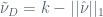
where upper triangular matrices contain the binomial coefficients and is the vector of unknown polynomial coefficients to be solved for in terms of the polynomial coefficients in the preceding dimension. Carrying the recursion out from the base case , the higher-dimensional lattice volumes are given by
where by inspection, the highest order coefficients decrease towards as increases. This is expected as the majority of the volume moves towards the origin as grows. For some context, we can compare the lattice volumes bounded under larger p-norms such as or Euclidean (see post on Gauss circle problem, volume appx. hypersphere) and the norm given by (lattice volume trivially ). By inspection, the lattice volume gap between and grows wider as the leading polynomial terms of decay to (see plot below).
This concludes our four-part foray into image-source models within high-dimensional integer lattice maps. If any new or interesting results come up or any errors found, I will update accordingly.
Notes: Animations generated in GeoGebra, equations and figures were from my draft paper.
[…] With the distance bound and Gauss circle problem out of the way, we will continue our investigation of lattice volume bounds in terms of the or taxi-cab distance in the next post. […]
[…] direct computation in these spaces is expensive but some clever maths [see tutorial (parts 1, 2, 3, 4)] reduced the asymptotic costs to the point of practical use (e.g. a Reverb plugin). Parameterizing […]


[…] to process individual image-sources within DSP pipelines (e.g. updating a tapped delay-line). See post. Related: linear algebra and dynamic […]
LikeLike
[…] With the distance bound and Gauss circle problem out of the way, we will continue our investigation of lattice volume bounds in terms of the or taxi-cab distance in the next post. […]
LikeLike
[…] direct computation in these spaces is expensive but some clever maths [see tutorial (parts 1, 2, 3, 4)] reduced the asymptotic costs to the point of practical use (e.g. a Reverb plugin). Parameterizing […]
LikeLike